BIOS 662 HW 2
Author:
ctn92
Last Updated:
12 anni fa
License:
Creative Commons CC BY 4.0
Abstract:
Personal template for typing of solutions to homework problems.

\begin
Discover why over 25 million people worldwide trust Overleaf with their work.

\begin
Discover why over 25 million people worldwide trust Overleaf with their work.
\documentclass[a4paper]{article}

\usepackage[english]{babel}
\usepackage[utf8]{inputenc}
\usepackage{amsmath,amsfonts}
\usepackage{graphicx}
\usepackage[colorinlistoftodos]{todonotes}
\usepackage[margin=1in]{geometry}
\usepackage{enumitem}

\title{BIOS 662 HW 2}

\author{Crystal Nguyen}

\date{\today}

\begin{document}
\maketitle

\section*{Problem 1}

\begin{enumerate}[label=(\alph*)]
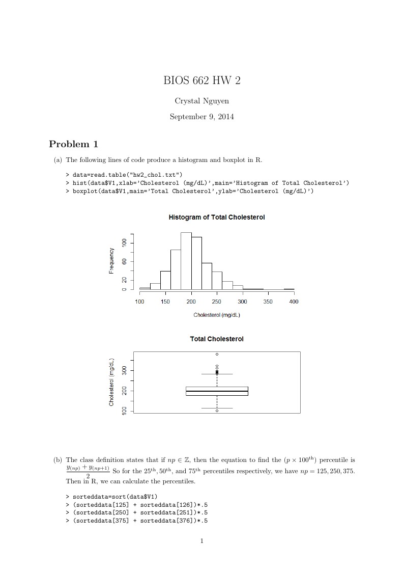
\item The following lines of code produce a histogram and boxplot in R.
\begin{verbatim}
> data=read.table("hw2_chol.txt")
> hist(data$V1,xlab='Cholesterol (mg/dL)',main='Histogram of Total Cholesterol')
> boxplot(data$V1,main='Total Cholesterol',ylab='Cholesterol (mg/dL)')
\end{verbatim}
\begin{center}
\includegraphics[scale=0.5]{Cholesterol_Histogram.png}\\
\includegraphics[scale=0.5]{Cholesterol_Boxplot.png}
\end{center}

\item The class definition states that if $np\in\mathbb{Z}$, then the equation to find the $(p\times 100^{\text{th}})$ percentile is $\dfrac{y_{(np)}+y_{(np+1)}}{2}$ So for the $25^{\text{th}},50^{\text{th}},$ and $75^{\text{th}}$ percentiles respectively, we have $np=125, 250,375$. Then in R, we can calculate the percentiles.
\begin{verbatim}
> sorteddata=sort(data$V1)
> (sorteddata[125] + sorteddata[126])*.5
> (sorteddata[250] + sorteddata[251])*.5
> (sorteddata[375] + sorteddata[376])*.5
\end{verbatim}
This produces the values $177.0,198.5,$ and $220.0$.
\begin{verbatim}
> quantile(data$V1, c(.25,.5,.75))
\end{verbatim}
then confirms the 25th, 50th, and 75th percentiles, respectively, to be $177.0, 198.5, 220.0$.

\item The interquartile range (IQR) is then said to be over $(177.0,220.0)$, or equal to $220.0-177.0=43.0$.

\item The $75^{\text{th}}$ percentile $+ 1.5 IQR$ is $220.0+1.5(43.0)=284.5$, and the $25^{\text{th}}$ percentile $- 1.5 IQR$ is $177.0-1.5*43.0=112.5$, Then we can find tthe observations greater than $1.5 IQR$ away from our interquartile range from the following code.
\begin{verbatim}
> which(sorteddata > 284.5)
> which(sorteddata < 112.5)
\end{verbatim}
This provides the index of the observations where the values outside $1.5 IQR$ are located. The first line returns the values $491$ through $500$, meaning that the greatest value smaller than the upper limit which we are searching for is indexed at $490$. Similarly, the second line returns only the value $1$, so we want to know the value indexed at $2$. So
\begin{verbatim}
> sorteddata[490]
> sorteddata[2]
\end{verbatim}
then returns $282$ and $114$, respectively. This appears to match with the boxplot previously returned. Since the values outside the $1.5 IQR$ range should be represented by the circles beyond the whiskers, we can count them to see if they match up to the number of values outside the desired range. The search for data points greater than $284.5$ returned $9$ values and there are $9$ circles above the upper whisker, this appears to match correctly. Similarly, the search for data below $112.5$ returned only $1$ data point, which can be associated with the single circle below the lower whisker.

\item The following code produces a boxplot to compare the distribution of total cholesterol, stratified by whether or not the individual experienced a CHD event.
\begin{verbatim}
> newsorteddata=data[order(data$V2),]
> boxplot(data$V1~data$V2,data=newsorteddata,xlab='Presence of CHD Event',ylab=
'Total Cholesterol',main='Cholesterol and CHD Event Boxplot')
\end{verbatim}
\begin{center}
\includegraphics[scale=0.5]{Comparison_Boxplot.png}
\end{center}
This comparison shows that those who did not experience a CHD event had total cholesterol levels with more spread and outliers, as seen by the whisker length and circles. These people also had a lower median total cholesterol, potentially suggesting that a lower cholesterol level will reduce the risk of a CHD event. Those who did experience a CHD event had less spread, with smaller whiskers, and the median total cholesterol was higher.

\end{enumerate}

\section*{Problem 2}

\begin{enumerate}[label=(\alph*)]
\item The following lines of code in R calculate the means and standard deviations for individuals who do and do not have hypercalcemia, respectively.
\begin{verbatim}
> data2=read.table('hw2_PGE.txt',head=T)
> mean(data2$iPGE[which(data2$Hypercalcemia>0)])
> sd(data2$iPGE[which(data2$Hypercalcemia>0)])
> mean(data2$iPGE[which(data2$Hypercalcemia==0)])
> sd(data2$iPGE[which(data2$Hypercalcemia==0)])
\end{verbatim}
These lines give the means to be $241.45$ and $147.5$ and the standar deviations to be $144.46$ and $46.17$. This is not conclusive evidence to say that the two means are different. The standard deviation iPGE for individuals with hypercalcemia is much too large and contains the mean for individuals without hypercalcemia inside of it.

\item
\begin{verbatim}
> plot(data2$iPGE,data2$Ca)
\end{verbatim}
produces the following plot.
\begin{center}
\includegraphics[scale=0.5]{iPGE_Ca_Scatter.png}
\end{center}
This scatter plot suggests there may exist some direct trend between iPGE and mean serum calcium, although there appears to be an extremely odd data point with less than $100$ iPGE, but $18$ mean serum calcium.

\item The odd data point from above happens to be patient $11$ with the lowest iPGE value at $60$ and $18$ mean serum calcium. I would suggest altering the calcium value to $9.2$, as the patient with the next lowest $iPGE$ has a calcium value of $9.2$, and I would assume that the outlier patient would have a calcium value of that or lower.
\item Altering this value would also alter the patients value for hypercalcemia from $1$ to $0$. Then the mean iPGE for patients with hypercalcemia would increase, and the standard deviation would decrease. Simultaneously, the mean iPGE for patients without hypercalcemia would decrease, and the standard deviation would increase. It is difficult to say without doing the calculations, but I think it is very possible that the means would appear to be very different as opposed to how they appeared before.


\end{enumerate}
\end{document}