Algorithm Lab Template
Author:
Roshan Pandey
Last Updated:
7 anni fa
License:
Creative Commons CC BY 4.0
Abstract:
Algorithm Lab Template
\begin
Discover why over 25 million people worldwide trust Overleaf with their work.
Algorithm Lab Template
\begin
Discover why over 25 million people worldwide trust Overleaf with their work.
\documentclass[0pt]{article}
\usepackage[margin=0.5in]{geometry}
\usepackage{listings}
\usepackage{pgfplots}
\usepackage{xcolor}
\lstset{
language = C,
frame=tb, % draw a frame at the top and bottom of the code block
tabsize=4, % tab space width
showstringspaces=false, % don't mark spaces in strings
commentstyle=\color{green}, % comment color
keywordstyle=\color{blue}, % keyword color
stringstyle=\color{red} % string color
}
\begin{document}
\begin{center}
\begin{LARGE}
\textcolor{red}{\underline{SORTING ALGORITHMS}}
\end{LARGE}
\\
\leavevmode \\
\end{center}
% Bubble Sort Starts here
\begin{flushleft}
\textbf{\textcolor{red}{1. Bubble Sort}}
\leavevmode \\
\begin{description}
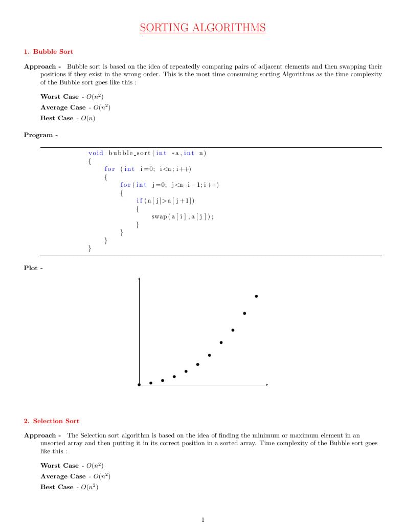
\item[Approach - ] Bubble sort is based on the idea of repeatedly comparing pairs of adjacent elements and then swapping their positions if they exist in the wrong order. This is the most time consuming sorting Algorithms as the time complexity of the Bubble sort goes like this :
\leavevmode \\
\begin{description}
\item[Worst Case] - \(O(n^2)\)
\item[Average Case] - \(O(n^2)\)
\item[Best Case] - \(O(n)\)
\end{description}
\leavevmode \\
\item[Program - ] \leavevmode \\
\leavevmode \\
\begin{lstlisting}
void bubble_sort(int *a,int n)
{
for (int i=0; i<n;i++)
{
for(int j=0; j<n-i-1;i++)
{
if(a[j]>a[j+1])
{
swap(a[i],a[j]);
}
}
}
}
\end{lstlisting}
\item[Plot - ] \leavevmode \\
\end{description}
\end{flushleft}
\begin{center}
\begin{tikzpicture}
\begin{axis}[
axis lines=middle,
xmin=0, xmax=11000,
ymin=0, ymax=0.6,
xtick=\empty, ytick=\empty
]
\addplot [only marks] table {
0 0
1000 0.009556
2000 0.02371
3000 0.04547
4000 0.074976
5000 0.113558
6000 0.165204
7000 0.236573
8000 0.305851
9000 0.399738
10000 0.49556
};
\end{axis}
\end{tikzpicture}
\end{center}
\leavevmode \\
% Bubble Sort Ends here
% Selection Sort Starts here
\begin{flushleft}
\textbf{\textcolor{red}{2. Selection Sort}}
\leavevmode \\
\begin{description}
\item[Approach - ] The Selection sort algorithm is based on the idea of finding the minimum or maximum element in an unsorted array and then putting it in its correct position in a sorted array. Time complexity of the Bubble sort goes like this :
\leavevmode \\
\begin{description}
\item[Worst Case] - \(O(n^2)\)
\item[Average Case] - \(O(n^2)\)
\item[Best Case] - \(O(n^2)\)
\end{description}
\leavevmode \\
\item[Program - ] \leavevmode \\
\leavevmode \\
\begin{lstlisting}
void selection_sort(int *a,int n)
{
for(int i=0;i<n-1;i++)
{
imin=i;
for(int j=i+1;j<n;j++)
{
if(a[j]<a[imin])
imin=j;
}
swap(a[imin],a[i])
}
}
\end{lstlisting}
\item[Plot - ] \leavevmode \\
\end{description}
\end{flushleft}
\begin{center}
\begin{tikzpicture}
\begin{axis}[
axis lines=middle,
xmin=0, xmax=11000,
ymin=0, ymax=0.6,
xtick=\empty, ytick=\empty
]
\addplot [only marks] table {
0 0
1000 0.003479
2000 0.013566
3000 0.027378
4000 0.041152
5000 0.062114
6000 0.085499
7000 0.119053
8000 0.143657
9000 0.180674
10000 0.22365
};
\end{axis}
\end{tikzpicture}
\end{center}
\leavevmode \\
% Selection Sort Ends here
% Insertion Sort Starts here
\begin{flushleft}
\textbf{\textcolor{red}{3. Insertion Sort}}
\leavevmode \\
\begin{description}
\item[Approach - ] Insertion sort is based on the idea that one element from the input elements is consumed in each iteration to find its correct position i.e, the position to which it belongs in a sorted array. Time complexity of the Bubble sort goes like this :
\leavevmode \\
\begin{description}
\item[Worst Case] - \(O(n^2)\)
\item[Average Case] - \(O(n^2)\)
\item[Best Case] - \(O(n)\)
\end{description}
\leavevmode \\
\item[Program - ] \leavevmode \\
\leavevmode \\
\begin{lstlisting}
void insertion_sort(int *a,int n)
{
for(int i=1;i<n;i++){
value = a[i];
hole =i;
while(hole>0&&a[hole-1]>value){
a[hole] = a[hole-1];
hole--;}
a[hole] =value;
}
}
\end{lstlisting}
\item[Plot - ] \leavevmode \\
\end{description}
\end{flushleft}
\begin{center}
\begin{tikzpicture}
\begin{axis}[
axis lines=middle,
xmin=0, xmax=11000,
ymin=0, ymax=0.6,
xtick=\empty, ytick=\empty
]
\addplot [only marks] table {
0 0
1000 0.003592
2000 0.009168
3000 0.019161
4000 0.029052
5000 0.039449
6000 0.055332
7000 0.068427
8000 0.089401
9000 0.113026
10000 0.135115
};
\end{axis}
\end{tikzpicture}
\end{center}
\leavevmode \\
% Insertion Sort Ends here
% Merge Sort Starts here
\begin{flushleft}
\textbf{\textcolor{red}{4. Merge Sort}}
\leavevmode \\
\begin{description}
\item[Approach - ] Merge sort is a divide-and-conquer algorithm based on the idea of breaking down a list into several sub-lists until each sublist consists of a single element and merging those sublists in a manner that results into a sorted list. Time complexity of the Bubble sort goes like this :
\leavevmode \\
\begin{description}
\item[Worst Case] - \(O(nlogn)\)
\item[Average Case] - \(O(nlogn)\)
\item[Best Case] - \(O(nlogn)\)
\end{description}
\leavevmode \\
\item[Program - ] \leavevmode \\
\leavevmode \\
\begin{lstlisting}
void merge_sort(int *a,int n)
{
int mid,*l,*r;
if(size==1) { return 1;}
mid = size/2;
l = new int [mid];
r = new int [size-mid];
for(int i=0;i<mid;i++) l[i] = a[i];
for(int i=mid;i<size;i++) r[i-mid] = a[i];
MergeSort(l,mid);
MergeSort(r,size-mid);
Merge(l,r,a,mid,size-mid);
}
\end{lstlisting}
\item[Plot - ] \leavevmode \\
\end{description}
\end{flushleft}
\begin{center}
\begin{tikzpicture}
\begin{axis}[
axis lines=middle,
xmin=0, xmax=11000,
ymin=0, ymax=0.01,
xtick=\empty, ytick=\empty
]
\addplot [only marks] table {
0 0
1000 0.000853
2000 0.001374
3000 0.00196
4000 0.002169
5000 0.003228
6000 0.005415
7000 0.007569
8000 0.00666
9000 0.0061199
10000 0.008269
};
\end{axis}
\end{tikzpicture}
\end{center}
\leavevmode \\
% Merge Sort Ends here
% Quick Sort Starts here
\begin{flushleft}
\textbf{\textcolor{red}{5. Quick Sort}}
\leavevmode \\
\begin{description}
\item[Approach - ] Quick sort is based on the divide-and-conquer approach based on the idea of choosing one element as a pivot element and partitioning the array around it such that: Left side of pivot contains all the elements that are less than the pivot element Right side contains all elements greater than the pivot Time complexity of the Bubble sort goes like this :
\leavevmode \\
\begin{description}
\item[Worst Case] - \(O(n^2)\)
\item[Average Case] - \(O(nlogn)\)
\item[Best Case] - \(O(nlogn)\)
\end{description}
\leavevmode \\
\item[Program - ] \leavevmode \\
\leavevmode \\
\begin{lstlisting}
void quick_sort(int *a,int start,int end)
{
int pIndex;
if(start<end)
{
pIndex=partition(a,start,end);
QuickSort(a,start,pIndex-1);
QuickSort(a,pIndex+1,end);
}
}
\end{lstlisting}
\item[Plot - ] \leavevmode \\
\end{description}
\end{flushleft}
\begin{center}
\begin{tikzpicture}
\begin{axis}[
axis lines=middle,
xmin=0, xmax=110000,
ymin=0, ymax=0.01,
xtick=\empty, ytick=\empty
]
\addplot [only marks] table {
0 0
10000 0.003608
20000 0.006167
30000 0.006628
40000 0.008968
50000 0.007334
60000 0.006411
70000 0.005522
80000 0.004264
90000 0.005855
100000 0.00607
};
\end{axis}
\end{tikzpicture}
\end{center}
\leavevmode \\
% Quick Sort Ends here
% Counting Sort Starts here
\begin{flushleft}
\textbf{\textcolor{red}{6. Counting Sort}}
\leavevmode \\
\begin{description}
\item[Approach - ] In Counting sort, the frequencies of distinct elements of the array to be sorted is counted and stored in an auxiliary array, by mapping its value as an index of the auxiliary array. Time complexity of the Bubble sort goes like this :
\leavevmode \\
\begin{description}
\item[Worst Case] - \(O(n+k)\)
\item[Average Case] - \(O(n+k)\)
\item[Best Case] - \(O(n+k)\)
\end{description}
\leavevmode \\
\item[Program - ] \leavevmode \\
\leavevmode \\
\begin{lstlisting}
void counting_sort(int *arr,int n,int RANGE)
{
int count[RANGE]={0};
int out[n];
for(i=0;i<n;i++) ++count[arr[i]];
for(i=1;i<RANGE;i++) count[i]+=count[i-1];
for(i=n-1;i>=0;i--){
out[count[arr[i]]-1]=arr[i];
--count[arr[i]];
}
for(i=0;i<n;i++) arr[i]=out[i];
}
\end{lstlisting}
\item[Plot - ] \leavevmode \\
\end{description}
\end{flushleft}
\begin{center}
\begin{tikzpicture}
\begin{axis}[
axis lines=middle,
xmin=0, xmax=110000,
ymin=0, ymax=0.05,
xtick=\empty, ytick=\empty
]
\addplot [only marks] table {
0 0
10000 0.001974
20000 0.016839
30000 0.004715
40000 0.020774
50000 0.009915
60000 0.02424
70000 0.015947
80000 0.032722
90000 0.023292
100000 0.040942
};
\end{axis}
\end{tikzpicture}
\end{center}
\leavevmode \\
% Counting Sort Ends here
% Heap Sort Starts here
\begin{flushleft}
\textbf{\textcolor{red}{7. Heap Sort}}
\leavevmode \\
\begin{description}
\item[Approach - ] Heaps can be used in sorting an array. In max-heaps, maximum element will always be at the root. Heap Sort uses this property of heap to sort the array.
\leavevmode \\
Consider an array \(Arr\) which is to be sorted using Heap Sort.
1) Initially build a max heap of elements in Arr.
\leavevmode \\
2) The root element, that is \(Arr[1]\), will contain maximum element of \(Arr\). After that, swap this element with the last element of \(Arr\) and heapify the max heap excluding the last element which is already in its correct position and then decrease the length of heap by one.
\leavevmode \\
3) Repeat the step 2, until all the elements are in their correct position.
Time complexity of the Bubble sort goes like this :
\leavevmode \\
\begin{description}
\item[Worst Case] - \(O(nlogn)\)
\item[Average Case] - \(O(nlogn)\)
\item[Best Case] - \(O(nlogn)\)
\end{description}
\leavevmode \\
\item[Program - ] \leavevmode \\
\leavevmode \\
\begin{lstlisting}
void heap_sort(int *a,int n)
{
for (int i = n / 2 - 1; i >= 0; i--)
heapify(arr, n, i);
for (int i=n-1; i>=0; i--)
{
swap(arr[0], arr[i]);
heapify(arr, i, 0);
}
}
\end{lstlisting}
\item[Plot - ] \leavevmode \\
\end{description}
\end{flushleft}
\begin{center}
\begin{tikzpicture}
\begin{axis}[
axis lines=middle,
xmin=0, xmax=11000,
ymin=0, ymax=0.03,
xtick=\empty, ytick=\empty
]
\addplot [only marks] table {
0 0
1000 0.00427
2000 0.001148
3000 0.006341
4000 0.004332
5000 0.010829
6000 0.010202
7000 0.016218
8000 0.016115
9000 0.022145
10000 0.019955
};
\end{axis}
\end{tikzpicture}
\end{center}
\leavevmode \\
% Heap Sort Ends here
\noindent\rule{\textwidth}{0.4pt}
\end{document}